The supplied factory compounds provide a good, generic starting point for many particle simulations. Since ICE was developed to replace the original XSI particles, the factory emitters follow many of the conventions for emission controls already established in the old paradigm. Anyone who has needed more precise control over emission parameters (e.g. emitting one particle from each vertex point of a source mesh), or something outside the box (e.g. emitting particles from only the edges of a mesh) has discovered quickly that the ICE factory emission compounds are somewhat limited in their powers.
Early advice from the developers and online community was to rely on the [Filter] and [Delete Point] nodes in tandem with the factory emission nodes as the primary solution for non standard emissions. While this technique provides more opportunities than default emissions, it is possibly bad advice. By exploring the workings of the factory emission nodes, one discovers that building emissions from scratch is actually quite simple since it requires only a few critical nodes. What's more, it is also possible to precisely construct a cloud by controlling exactly where and how new particles are created, which is more efficient than creating a huge cloud and filtering out unwanted chaff.
The following tutorials will walk step-by-step through setting up custom particle emissions in ICE. Please note the following conventions, established for the sake of brevity:
1) Instructions on building ICE Trees will refer only to node and compound names such as [Delete Point] rather than listing the explicit address in the node library such as Tool>Point Cloud>Delete Point. This is done under the assumption that the user can quickly find the nodes by typing their names in the node search field.
2) A sentence describing the creation and connection of nodes will be written in the following shorthand:
Connect a new [3D Vector]:Result→ ¤Port1:[ICETree]
- Square brackets denote the name of a node, such as [3D Vector]
- A colon after the node bracket is used to denote an output port, such as [3D Vector]:Result
- A colon prior to the node bracket is used to denote an input port, such as Port1:[IceTree]
- The "→ ¤" symbols are used to denote a connection line
- In a new XSI scene, do Get>Primitive>Point Cloud>Empty
- Open an ICE Tree window and do Create>Simulated ICE Tree
- Connect a new [Add Point] :Add → ¤Port1:[ICETree]
- Connect a new [3D Vector]:Result→ ¤Positions1:[Add Point]
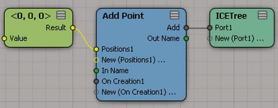 |
| Figure-1:ICE Tree |
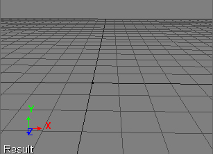 |
| Figure-2: A single black dot visible at origin |
This ICE Tree is as simple as particle systems can get. It emits a single particle per frame where each particle has no properties other than a 3D vector for the point position, which we left at the default setting of (0,0,0). The particles are represented as a static black dot at origin because they have no color, size, shape, or velocity.
Let's add some animation to the [3D Vector] so we can see each particle that gets emitted:
- Set the Play Control frame to 1
- Double-click on the [3D Vector Node] and set keys on the X and Y parameters
- Set the Play Control frame to 100
- Set the X and Y parameter values to 10, and set keys on both
- Play the animation
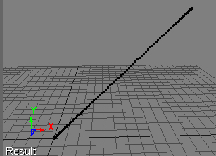 |
| Figure-3: Single particle per frame from animated input |
Based on this very simple ICE Tree, we can start to see how the [Add Point] node works for a simulated ICE Tree. It uses input position information to add new points to the cloud at each frame of animation. We can add more particles per frame by adding more [3D Vector] nodes and expanding the Position inputs on the [Add Points] node (see figure-4).
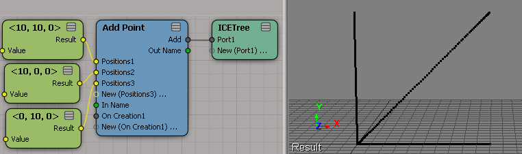 |
| Figure-4: Additional [3D Vector] nodes with different animated values create more particles per frame |
We can also input an array of point positions or locations from any source into a Position input of the [Add Point] node (see figure-5).
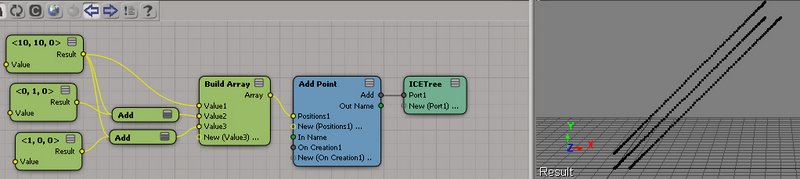 |
| Figure-5 A custom array is constructed using the original animated [3D Vector] node. Additional members of the array are created by adding values to the original vector and feeding them into the [Build Array] node |
Keep in mind, without any additional information, the created particles represent nothing more than a location in space. They will not render, they will not react to forces, and they won't stop generating new points at every frame. Gaining control over these other aspects requires the addition of more nodes to the tree (Of course, not every particle sim we create needs to be rendered, or react to forces, so it's good to know by creating an emission setup from scratch we can leave out extraneous information).
Lesson 2: Adding Basic Particle Attributes
- Start with the results from the above exercises
- Insert an [Emit From Surface] node into the ICE Tree
- Mouse over the [Emit From Surface] node and you should see an 'e' in a circle pop up at the top left of the node. Click on this button to explore inside this factory compound. The insides will look like figure-6.
- Select the two brownish nodes in the upper left of the compound, [Init Particle Data] and [Init Force and Velocity] and copy them into the memory buffer (CTRL-C).
- Exit the inside of the compound by clicking on the little x in the box on the upper left of the compound interior interface.
- Delete the [Emit From Surface] compound node.
- Paste the two nodes copied from the inside into the ICE Tree (CTRL-V).
- Connect [Init Particle Data]:Execute→ ¤On Creation1:[Add Point]
- Connect [Init Force and Velocity]:Execute→ ¤New (On Creation 1):[Add Point]
- Double-Click on the [Init Particle Data] node (notice the PPG has many of the attributes you would set for a default factory particle emission. This is not a coincidence considering that's where we just grabbed it from!)
- Set the shape attribute to sphere.
- Run the Playback.
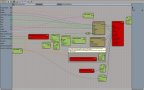 |
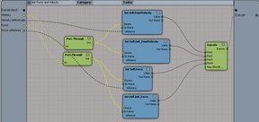
| Figure-6: The [Emit From Surface] node internals |
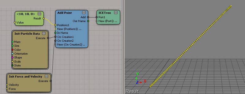 |
| Figure-7 [Init Particle Data] and [Init Force and Velocity] nodes salvaged from factory [Emit From Surface] compound |
From Figure-7 we can see that our particles now have color and size, along with all the other attributes that were set by the [Init Particle Data] node. From the [Init Force and Velocity] node, our particles also get all the necessary attributes for using factory forces in simulation.
This would be a good time to explore what's inside both of these compounds.
 |
 |
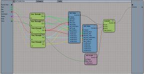
| Figure-8: [Init Paritcle Data] node internals | Figure-9: [Init Force and Velocity] node internals |
The internals of both nodes aren't very complicated at all. In fact, they are made up almost entirely of [Set Data] nodes. Both compounds set particle attributes, along with a partner Init_attribute. The Init_attribute stores the values at creation time, while the rest of the attributes are used during simulation to evolve over time. Keep this technique in mind when you need to create your own custom attributes. It can be important to know, for example, what your original orientation was, since you might need your particle to wobble but not get too far from its original rotation.
Notice that things are starting to look more like the default emission controls? We're already at a starting point for simulation work, and it required very few nodes and very little work to get here.
Lesson 3: Controlling Emission Timing
- Start with the ICE Tree from the end of Lesson 2.
- Add an [If] node into the ICE Tree.
- Connect [Add Point]:Add→ ¤If True:[If]
- Connect [If]:Result→ ¤Port1:[ICETree]
- Add a [Test Current Frame] node into the ICE Tree.
- Connect [Test Current Frame]:Result→ ¤Condition:[If]
- Double-Click on the [Test Current Frame] node
- Set the Test Frame parameter value to 50
- Set the Compare Type parameter to Less Than or Equal To
- Run the Simulation
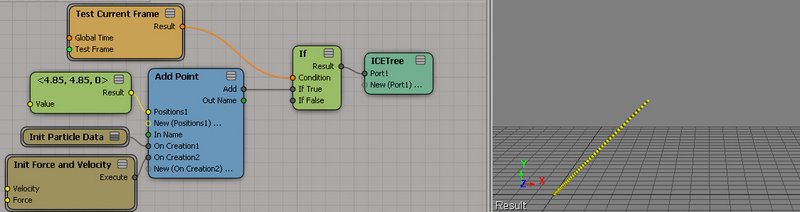 |
| Figure-10 Frame Test switch added to graph to control particle emission timing |
Controlling when the emission should start and stop is as simple as adding a simple switch using an [If] statement. In this case, we are testing that the current frame is less than or equal to 50. When this condition is true, the [Add Point] node executes. When false, it sits idle. For certain kinds of emissions, we will want to emit all points on a single frame, often the very first one of the animation. This same setup works nicely for that. Keep in mind, however, that points are generated at the end of a frame, so you may need to add an extra frame at the beginning of your scene. For example, if you want to create points only on frame 1, make sure to set the scene start frame to 0.
Of course, you can use any test you like to control the switch for adding points. You could add points every other frame by testing the remainder when you divide the current frame by 2, or using boolean logic([And] nodes and [Or] nodes), emit particles between multiple frame ranges.
Lesson 4: Emitting Particles from Vertex Points
- Start with your ICE Tree from Lesson 3
- Set the Test Frame parameter on the [Test Current Frame] node to 100 so that particles are added for the entire animation
- Model>Get>Primitive>Polygon Mesh>Torus
- Set keys on translation and rotation at origin, at frame 1
- Set the frame to 100
- Translate the torus to the upper right side of the view, store the keys
- Rotate the torus 2-3 full times in a couple of axes. Your resulting animation should resemble figure-11
- From an explorer view, drag and drop the torus into the ICE Tree. This should come into the tree as a [Get torus] node, which is just a Get Data node that is pointing at the torus.
- Add another [Get Data] node to the ICE Tree
- Connect [Get torus]:Out Name → ¤In Name:[Get Data]
- Double-Click on the [Get Data] node and click on the Explorer button. Expand the Polygon Mesh node in the pop up explorer and select PointLocation. The node should change its name to [Get..PointLocation]
- Connect [Get..PointLocation]:Value→ ¤Positions1:[Add Point].
- If your ICE Tree looks like figure-12, go ahead and run your simulation.
| Figure-11: Simple animation of torus |
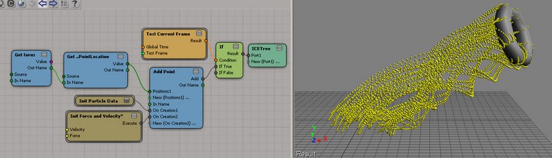 |
| Figure-12: ICE Tree and resulting simulation |
Lesson 5: Emitting Particles from Edges, Polygons, and other Data Sources
In Lesson 4, we used PointLocation data from an input torus to emit particles for our cloud. When pulling PointLocation information into an ICE Tree, it automatically converts its SRT space relative to the SRT space of the ICE Tree host node, in this case the particle cloud. If we were to pull PointPosition data from the torus instead, [Add Point] would still add new particles to the cloud, but they would all be situated around the origin. You can try this by going back to step-11 of Lesson 4 and selecting PointPosition instead of PointLocation. You can also try EdgePosition, PolygonPosition, PointNormal, and any other attribute from the torus that is a 3D Vector data type. [Add Point] will work with any of them.
However, in order to emit the points relative to the torus, we have to do a little more math. We need to get the global SRT from the torus and multiply it by the data we are pulling from the torus. The result will be reflected in global space relative to where the torus is:
- Starting with the ICE Tree from Lesson 4, double-click on the [Get Data] node connected after the [Get torus] node and select the EdgePosition attribute. The node will change names to [Get ..EdgePosition].
- Run the simulation to see that particles are all emitted around the origin
- Add a new [Get Data] node to the ICE Tree
- Connect [Get torus]:Out Name → ¤In Name:[Get Data]
- Double click on the new [Get Data] node and set the reference parameter to "kine.global" (without the quotation marks). The node name will change to [Get .kine.global].
- Add a [Multiply Vector by Matrix] node to the ICE Tree.
- Connect [Get ..EdgePosition]:Value→ ¤Vector:[Multiply Vector by Matrix]
- Connect [Get .kine.global]:Value→ ¤Matrix:[Multiply Vector by Matrix]
- Connect [Multiply Vector by Matrix]:Result→ ¤Positions1:[Add Point]
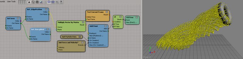 |
| Figure-13 ICE Tree for emitting particles from Edge Position data. Results on the right. Image links to an enlarged view. |
You may now change the data set pulled from the torus to any of the other 3D Vector sets, such as PointPosition and PolygonPosition, and they will emit particles relative to the center animation of the torus in the scene.
Lesson 6: Emitting Particles From Surfaces and Volumes
- Start with the ICE Tree from Lesson 5
- Delete the two Get Data nodes that are connected to the [Get torus] node, [Get ..EdgePosition] and [Get .kine.global].
- Delete the [Multiply Vector by Matrix] node.
- Add a [Generate Sample Set] node to the ICE Tree.
- Connect [Get torus]:Value→ ¤Geometry:[Generate Sample Set].
- Connect [Generate Sample Set]:Samples→ ¤Positions1:[Add Point].
- Double-click the [Generate Sample Set] node and set the Rate Type to Number per Frame.
- Run the simulation and check the results against Figure-14.
 |
| Figure-14 ICE Tree for emitting particles from random points on surface. Results on the right |
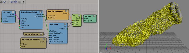
Notice the options inside the [Generate Sample Set] node. They allow you to set the rate of sampling per frame, second, or density. The resulting particles added to the point cloud are sampled randomly from the input geometry per frame. At this point the functionality of our simple node tree is almost identical to the factory [Emit From Surface] node, and our tree isn't very complicated at all.
We can drive a dynamic particle sim from here by simply adding forces and a [Simulate Particles] node to the input ports of the [ICETree] node (See Figure-15, 16).
 |
| Figure-15: ICE Tree with simulation nodes added |
| Figure-16: Resulting Simulation |
Lesson 7: Emitting From Custom Geometry Queries
We know how to emit from vertex points and other data sources from geometry input. We also know how to sample sets of random points using [Generate Sample Set]. So we can do what the factory emission nodes already do. The main point of this tutorial was to take us step-by-step until we could match the power of the factory emission compounds and ultimately move beyond them. Here we go.
- Start with the ICE Tree from Lesson 6.
- Delete the [Get torus] node and the [Generate Sample Set] node from the tree.
- Delete the torus from the scene.
- Double-click on the [Test Current Frame] node and set the Test Frame to 2 and the Compare Type to "Equal To".
- Model>Create>Text>Planar Mesh
- Type some text in a font you like at 48 points in size, and create the mesh
- Drag and drop the mesh node from an explorer into the ICE Tree. This will come in as Get Data node named [Get polymsh].
- Model>Get>Primitive>Point Cloud>Grid
- Rotate the Point Cloud grid by 90 degrees in x, then size it to fit over the text (see Figure-17)
- Translate the Particle Cloud Grid slightly forward in z space to position it in front of the text mesh.
- Increase the subdivisions of the Particle Cloud Grid for more coverage of the text.
- Drag and Drop the Particle Cloud Grid from an explorer view into the ICE Tree. This will come in as a node named [Get grid].
- Hide the Particle Cloud Grid.
- Add a new [Get Data] node to the ICE Tree.
- Connect [Get grid]:Out Name→ ¤In Name:[Get Data]
- Set the reference of the [Get Data] node to PointPosition. The name will change to [Get ..PointPosition]
- Add another [Get Data] node to the ICE Tree and connect [Get grid]:Out Name→ ¤In Name:[Get Data].
- Set the reference of the new [Get Data] node to ".kine.global" (without the quotation marks). The name will change to [Get .kine.global].
- Add a [Multiply Vector by Matrix] node to the ICE Tree.
- Connect [Get ..PointPosition]:Value→ ¤Vector:[Multiply Vector by Matrix]
- Connect [Get .kine.global]:Value→ ¤Matrix:[Multiply Vector by Matrix]
- Add a [Raycast] node to the ICE Tree.
- Connect [Get polymsh]:Value→ ¤Geometry:[Raycast]
- Connect [Multiply Vector by Matrix]:Result→ ¤Position:[Raycast]
- Connect [Raycast]:Location→ ¤Positions1:[Add Point]
- Double-click the [Raycast] node and set the Direction Z to -1.
- Step the Play Control frame from 1 to 2.
- Adjust the size of the particles and density of the Point Cloud Grid to taste. See Figure-18 for the Tree and results.
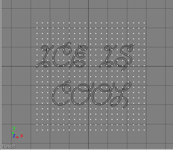 |
| Figure-17: Text mesh with Particle Cloud Grid |
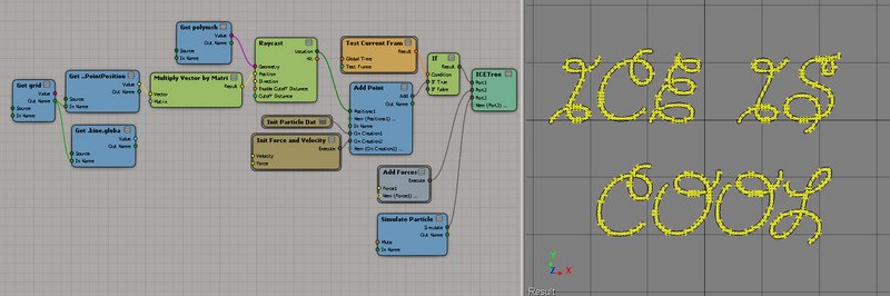 |
| Figure-18 ICE Tree using Raycast from a Point Cloud Grid onto a text mesh for particle emissions |
There are many more steps in the tutorial above, but most of them pertain to setting up the text mesh and the Particle Cloud Grid object. Looking at the node graph in Figure-18 you can see that it isn't very large or complex at all. The source for the emission data are points from the Particle Cloud Grid wherever they successfully raycast onto the text mesh.
There are some distinct advantages to setting up a Particle Emission using a point cloud primitive. You can see the density and location of the emission distribution prior to particle creation. You can also move or delete points on the Particle Cloud that is being sampled, or apply other deformation operators to that cloud such as point randomization. Ultimately, you have a very visually precise source for your emissions.
The same basic technique can be used, for example, with a Point Cloud Cube, shrink wrapped onto a spherical mesh. Instead of using the [Raycast] node, you can use [Get Closest Location]. This is one way to generate an even distribution of particles on a surface mesh (see Figure-19).
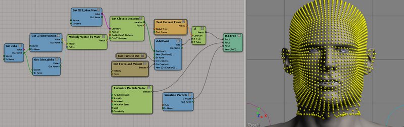 |
| Figure-19 A Primitive Point Cloud Cube is shrink wrapped over the man's head, and then used as a Point Position source for a [Get Closest Location] node. The resulting particle distribution is on the right. |
As with the text example, the density of the sampled Point Cloud can be adjusted after the fact, along with editing point positions, deleting unwanted points, applying randomization, etc.
Conclusion and Summary
Once understood, setting up custom emissions in ICE are a simple prospect. The critical nodes are [Add Point] along with initializing particle data, which can be quickly salvaged from the existing factory emission nodes.
[Add Point] will accept input from any source for PointLocations or 3D Vector data which is used as PointPosition data.
PointLocations automatically convert their coordinate space to the SRT of the ICE operator, but often we need to use input data from sceneobjects that have been transformed. We can convert these data sets to global space by multiplying their global SRT matrices by their input point vector data using a [Multiply Vector by Matrix] node.
Lastly, some of the types of distributions shown simply cannot be achieved easily or efficiently using the combination of factory emission nodes with filters. Building a new emission from scratch allows us to filter data before it enters the cloud, rather than emitting a massive cloud, then deleting unwanted or filtered points.